Partial equilibrium is a condition of economic equilibrium which takes into consideration only a part of the market, ceteris paribus, to attain equilibrium.

As defined by George Stigler, "A partial equilibrium is one which is based on only a restricted range of data, a standard example is price of a single product, the prices of all other products being held fixed during the analysis (Jain, 2006).

The supply and demand model are a partial equilibrium model where the clearance on the market of some specific goods is obtained independently from prices and quantities in other markets. In other words, the prices of all substitutes and complements, as well as income levels of consumers, are taken as given. This makes analysis much simpler than in a general equilibrium model which includes an entire economy.

Here the dynamic process is that prices adjust until supply equals demand. It is a powerfully simple technique that allows one to study equilibrium, efficiency and comparative statics. The stringency of the simplifying assumptions inherent in this approach make the model considerably more tractable, but may produce results which, while seemingly precise, do not effectively model real-world economic phenomena.

Partial equilibrium analysis examines the effects of policy action in creating equilibrium only in that particular sector or market which is directly affected, ignoring its effect in any other market or industry assuming that they are being small will have little impact if any. Hence this analysis is considered to be useful in constricted markets.

Léon Walras first formalized the idea of a one-period economic equilibrium of the general economic system, but it was French economist Antoine Augustin Cournot and English political economist Alfred Marshall who developed tractable models to analyse an economic system.

Assumptions:

1. Commodity price is given and constant for the consumers.
2. Consumers' taste and preferences, habits, incomes are also considered to be constant.
3. Prices of prolific resources of a commodity and that of other related goods (substitute or complementary) are known as well as constant.
4. Industry is easily availed with factors of production at a known and constant price compliant with the methods of production in use.
5. Prices of the products that the factor of production helps in producing and the price and quantity of other factors are known and constant.
6. There is perfect mobility of factors of production between occupation and places.
7. The above-mentioned points relate to a perfectly competitive market but can be further extended to monopolistic competition, oligopoly, monopoly and monopsony markets (Jhingan, 2007).

Applications of partial equilibrium discusses, when does an individual, a firm, an industry, factors of production attain their equilibrium points:

1. A consumer is in a state of equilibrium when they achieve maximum aggregate satisfaction on the expenditure that they make depending on the set of conditions relating to his tastes and preferences, income, price and supply of the commodity etc.
2. Producers’ equilibrium occurs when they maximize their net profit subject to a given set of economic situations.
3. A firm's equilibrium point is when it has no inclination in changing its production.

The minimum conditions of equilibrium:

In the short run:

Marginal Revenue = Marginal Cost.

In long run:

Marginal Cost = Marginal Revenue = Average Revenue = Long run Average Cost

It means that a firm is earning only a "normal profit" and has no intension to leave the industry. Equilibrium for an industry happens when there is normal profit made by an industry It is such a situation when no new firm wants to enter into it and the existing firm does not want to exit.

Only one price prevails in the market for a single product where the quantity of goods purchased by a buyer = total quantity produced by different firms. All the firms produce till that level where:

Marginal Cost=Marginal Revenue

In addition, the sails of the product at market price ruling at that point of time (Wikipedia, 2018). 

Factors of production, i.e., land, labour, capital, and entrepreneurs are in equilibrium when they are paid the maximum possible so as maximize the income. Here the Price = Marginal Revenue Product.

At this price it does not have any enticement to look for employment anywhere else.

The quantity of factors which its owners want to sell should be equal to the quantity which the entrepreneurs are ready to hire.

Limitations

• It is restricted to one particular portion of the economy.
• It lacks the ability to study the interrelations of all the parts of the economy.
• This analysis will fail if the improbable assumptions, which disconnect the study of specific market from the rest of the economy, are not taken into consideration.
• It has been unsuccessful in explaining the outcome of economic disturbance in the market that leads to demand and supply changes, moving from one market to another and thus instigating second- and third-order waves of change in the whole economy.

In partial equilibrium the welfare effects on consumers who purchase and the producers who produce in the market is distinguished by consumer surplus and producer surplus.

Consumer surplus

The amount that a consumer is ready to pay for a particular good minus the amount that the consumer actually pays. The amount that the consumer is willing to pay has to be greater (Suranovic, 2004).

In the graph given here, P1 is the price that a consumer is ready to pay for a particular product. But the producer may reduce the price to P2 expecting that either more people would buy at the reduced rate, or the person who was ready to pay P1 will purchase more of the same. The producer may further reduce the price to P3, again expecting more buyers or the same buyers purchasing more (Suranovic, 2004)

The price keeps on falling until P’, where the demand and the supply curves intersect: their intersection is the equilibrium point. Hence the consumer surplus for first consumer can be calculated as P1 - P’, decreasing for the second consumer to P2 - P’, and so on. Thus, the total consumer surplus in the market can be obtained by summing up the three rectangles. The triangle with the purple outline to the left indicates that area (Suranovic, 2004)

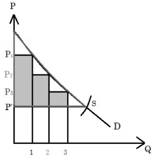
Figure 1. Consumer Surplus in the market

Figure 1 showing Consumer Surplus in the market, P refers to Price on the Y-axis, Q-refers to Quantity on X-axis, D-Demand Curve, S-Supply Curve.

Amount that a producer finally receives by selling a particular product minus the amount the producer is ready to accept for that good. The amount that the producer receives should be greater (Suranovic, 2004).

If only one unit of the commodity was demanded at the price P1, this becomes the price which the producer expects to receive. But if two units are demanded, the minimum price at which the producer would be ready to increase the supply shifts to P2. This continues and the final price that ultimately prevails in the market is P’, the price which is obtained by the intersection of the demand and supply curve in the market. The producer's surplus here would be initial price minus the final price. And total consumer surplus in the market will be summation of the three rectangles (Suranovic, 2004).

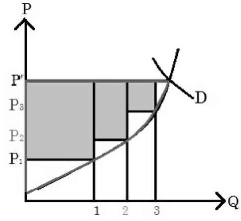
Figure 2. Producer Surplus in the market

Figure 2 showing Producer Surplus in the market, P refers to Price on the Y-axis, Q refers to Quantity on X-axis, D- Demand Curve, S-Supply Curve. As against partial equilibrium analysis, general equilibrium analysis is concerned with economic system as a whole. It recognizes the fact that economic system is a network in which all the parts are mutually dependent on one another and in mutual interaction with one another.

Goods are either competitive or substitutes. Some goods are used in the manufacture of other goods. Factors of production are complementary to each other to the extent they can be substituted for each other, they are competitive also. Resources also face competitive demand from producers.

Therefore, change in the demand or supply of any commodity or factor of production sets in motion a chain reaction. A disturbance in one sector of the economy produces its repercussions on all sides. General equilibrium analysis is concerned with the overall effects of a disturbance.

Instead of taking only a few variables at a time, we take into consideration all the relevant variables which may affect the particular phenomenon in hand. In this type of analysis, all the side-effects of an economic disturbance are analysed in full.

An example will make the concept of general equilibrium clearer. Suppose the demand for India-manufactured consumer goods suddenly increases in Western Europe. Indian exports will increase thereby increasing output, employment and profits in the export industries. Resources will be diverted from other industries to the export industries.

The demand and prices of the substitute commodities will also increase. The increased demand for exports will have economy-wide effects. An all-round analysis of the repercussions of the economic disturbance increased demand for manufactured consumer goods for export can be done only through general equilibrium theory.

General equilibrium analysis deals with the equilibrium of the whole organisation in the economy consumers, producers, resource-owners, firms and industries. Not only should individual consumers and firms be in equilibrium in themselves but also in relation to each other.

Business firms enter product markets as suppliers, but they enter factor markets as buyers. Households, on the other hand, are buyers in product markets but suppliers in factor markets. General equilibrium prevails when both the product and factor markets are in equilibrium in relation to each other.

General equilibrium analysis serves many important purposes.

Firstly, it provides us with a theoretical tool to understand the economy in its entirely the mechanics of its working, it structure, and the major forces making it work. The theory is analysis of the interrelationships of the various sectors of an economy. As such, it helps us in knowing clearly the economy-wide implications of an economic change.

Secondly, we can apply general equilibrium theory to determine the primary, secondary and tertiary effects of an economic disturbance which has an intersectoral impact. Whenever there is an economic disturbance say, like the defence programmes in the wake of Chinese aggression in 1962 it has some immediate effects in one sector of the economy.

Gradually, the impact of such a disturbance is felt in other sectors. The whole economy goes into disequilibrium. Process of adjustment to the economic disturbances starts to establish a new equilibrium.

As Richard Leftwich put it, “First comes the big splash from the disturbance. Particular equilibrium analysis handles the splash. But waves and then ripples are set up from it, affecting one another and affecting the area of the splash. The ripples run farther and farther, becoming smaller and smaller, until eventually they dwindle away. The tools of general equilibrium are required for analysis of the entire series of readjustments”.

Thus, general equilibrium theory is of great value in stressing the interdependence of various parts of the economic system, which is easily lost sight of in the use of partial equilibrium theory in micro-economic analysis.

Failure to recognise this interdependence is responsible for many errors in popular reasoning on economic policy.

The practical importance of general equilibrium analysis cannot be questioned. Recently, it has proved extremely useful in different forms:

1. The general equilibrium theory is being put to extensive use in the study of the development and other major programmes of modern economics to ascertain their feasibility, their impact and requirements. Take, for example, the effect of defence preparations to meet the Chinese threat.

It meant a rearrangement of all the priorities. There was heavier demand for steel and other construction materials, as also the demand for woollens.

It also meant heavier imports. Prices of all these commodities increased, diverting resources to these industries and away from some others. Eventually, effects were felt over the entire economy. An assessment of the full impact of such a programme in advance could be possible only through general equilibrium analysis.

2. Professor Wassily Leontief accomplished the task of bringing general equilibrium theory to the practical level by building his input-output analysis. The use of computers and other high-speed calculating machines has made it possible for us to solve hundreds of equations to find out a solution.

Thus, input-output analysis has been put to a variety of uses. Since this analysis can throw light on the structure of an economy and the interdependence between its different parts, it has been extensively used in planning for smooth growth of the national and international economy.

3. General equilibrium analysis has found its most extensive use in welfare economics. In this branch of economics, we study the ‘best’ allocation of resources, given the objectives of society. The search for such an organization of the economy leads us to apply the methods of general equilibrium.

4. Monetary theory and policy have been revolutionised by the introduction of general equilibrium analysis. It is now widely recognized that a meaningful monetary policy must apply to all the assets in the economy which are related to all the goods, capital and labour markets. Such a monetary policy is nothing but a study of general equilibrium effects of government policy.

Table 3. Difference between Partial and General Equilibrium

Partial Equilibrium	General Equilibrium
• Developed by Alfred Marshall.	• Leon Walras was first to develop it.
• Related to single variable	• More than one variable or economy as a whole is taken into consideration
• Based on two assumptions: Ceteris Paribus Other sectors are not affected due to change in one sector.	• It is based on the assumption that various sectors are mutually interdependent. There is an effect on other sectors due to change in one.
• Other things remaining constant, price of a good is determined	•Prices of goods are determined simultaneously and mutually. Hence all product and factor markets are simultaneously in equilibrium.